|
BAPI’s sensors may not have made it into space as yet, but they are now helping the US Government in its study of the solar system and cosmos and even in its search for ET. The Jet Propulsion Laboratory, a division of NASA, recently chose BAPI’s immersion sensors for integration into its Deep Space Network systems. Specifically, the sensors will be used in the guidance platform mechanism for the giant antennas in the California desert.What exactly is the Deep Space Network? |
Ruskin Products Now Offered with an Extended Limited Warranty!
Ruskin announces the extension of its limited warranty program from one year to five years from the date of delivery. Effective Feb. 1, 2017, the new warranty terms apply to all Ruskin products and are intended to inspire confidence in the Ruskin
“We are excited to offer this improved level of coverage to our customers,” said Mark Saunders, director of sales and marketing at Ruskin. “The move from one to five years demonstrates our commitment to quality and should reinforce and bolster the confidence our customers already have in the performance of our products. Additionally, engineers will find it easier to specify Ruskin products, especially when they are able to offer their customers this extended coverage.”
For additional information about the Ruskin sales policy and warranty program, please visit this link: Read Press Release.
Kele upholds warranty policies of its manufacturers.
The Power of One – Your Solution for Multiple Needs!
It’s summer; it’s time for grilling and outdoor parties! Imagine you are having your friends over to celebrate the big holiday. Your checklist includes a stop at the local meat market, the speciality hardware store to grab coal for your Big Green Egg, the grocery store to pick up beverages and the pool store to grab new floats.
We see this scenario in Business to Business situations – whether your sourcing from multiple suppliers, the current supplier is out of stock, doesn’t have the right brands, or just doesn’t carry the part you need – you may find yourself shopping with multiple suppliers. Working with Kele saves you multiple stops and gives you back your time! Our in-stock inventory includes 1.8 million parts that can ship same day and straight to your job site! We offer all the major brands and hard to find parts. There is no need to place several different purchase orders with multiple suppliers, which customers tell us can result in $25-$100 in additional costs per order. If you can eliminate even one additional purchase order, then you have saved your company at least $25 and freed up your time!
You are our number one priority. If you want it, then we want to stock it. The next time you have a list of material to purchase, come to us first! Shop at kele.com today!
Build the Perfect Panel

Did you know that Kele has a team of professionals dedicated to ensuring that your panels are built with 0 mistakes?
We have discovered that as many as 95% of the submitted panel layouts need adjusting in order to meet the customer’s stated needs?
Over our 30+ year history, our panel experts have found two general areas with regard to panel layouts that make up as much as 95% of the changes required to ensure correct panel operation. This is why Kele has a dedicated team that provides value-added services on the front end, such as “No Charge” panel review of your submitted diagrams, in order to ensure your panel operates the way you expect it to – flawlessly.
So, what are the two most common areas that we have identified that can cause failure in the field? Read more
From Loyal Customer to Proud Leader
Meet Richard Campbell, Kele’s CEO & President

Richard Campbell joins Kele, Inc. as President & CEO after years of being a customer. As a customer, Kele made Richard’s job easier with 1.8 million parts in-stock, same-day shipping and technical support. When he got the call to join the Kele team, he was excited about the opportunity.
Richard has walked in your shoes. He worked with commercial and industrial products at Ingersoll Rand for over 30 years, 27 of which were spent with the Trane brand focused on HVAC systems and building automation.
“I was blown away by the Kele teams’ passion for the customer,” said Richard.
“Kele makes it easy, allowing you to save time and focus on the things that are important to your customers. No matter how you want to buy, Kele is there for you,” said Richard.
Coming soon are additional value-added solutions to simplify your job.
Easily Configure Valve Sizes Fast!
Taking time to size a valve correctly saves you time, money and yourself a headache!
Picking the right size leads to performance
Our goal is to find the valve with the best control for your specific application. The Cv, or coefficient of flow of the valve, plays a big part in the valve’s performance. A valve that is sized correctly has accurate flow control, lasts beyond its expected life span and does not leak.
All you need to size a valve is the GPM and pressure drop! Calculate the Cv with this equation:
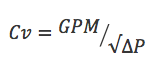
CV = coefficient of flow, GPM = flow rate in gallons per minute and ∆P = differential pressure
Selecting the wrong size results in complications
When a valve is too small, you won’t get enough flow, and the system will be forced to compensate by raising the head pressure of the pump. This causes higher differential pressure across your valve. The sudden drop in pressure causes cavitation and affects the life of the valve. The vibration and turbulence wears out the seals, which results in leaks.
Did you know most engineers oversize a pump by as much as 15% to cover for this type of mistake? Read more
Big Bertha, Our Largest Panel to Date

Kele has completed its largest scale panel to date through our own custom panel shop. Those at Kele lovingly referred to “her” as “Big Bertha” during the build. Dorsett Technologies of North Carolina partnered with us for a project to automate water pump functionality for their customer. Their 96”x72” panel was custom for several reasons, and we were glad to have them select Kele. Through our supplier relationships and white glove service, Dorsett received their gigantic panel without incident and had a completely successful install. Kele was chosen to create Bertha because:
- We conduct a 35-point inspection on all plans before the build.
- Our reputation for a cleanly wired panel proceeds us.
- We offer white glove shipping provisions.
- Our ability to incorporate specialty features not currently carried in our inventory.
Kele, specializes in special requests and getting a job done right. Dorsett Technologies expressly selected Kele for our clean wiring, ability to incorporate special parts and features, and our ability to customize the shipping. Their panel, a 96” X 72” enclosure complete with 6 controllers and all of the peripherals was specially constructed for their water pump station project. Additionally, Kele received and incorporated a touchscreen on the outside, mounted in the door. Dorsett has a close relationship with their enclosure partners, Austin Enclosures Co. Kele doesn’t typically carry their materials, but what the customer wants, the customer gets! Kele’s panel team worked with Austin Enclosures to meet the job’s specifications and received the large enclosure to complete the build. This was the first of series of panels that were needed.
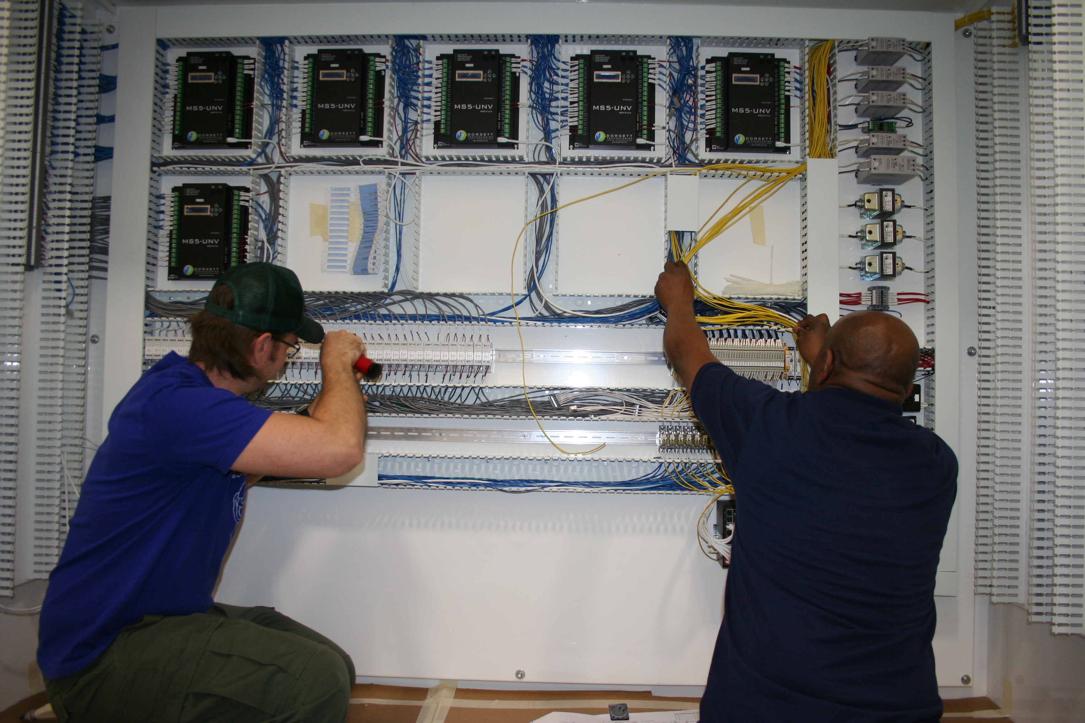
Since Kele had not done a 5’x 8’ panel that weighed 1,500 lbs. before, we sat down to establish what made this extraordinary. Our number one concern: SAFETY.
“The safety of our techs and taking care of the customers’ product are my utmost concern,” Lisa Bennett, Panel Shop Manager expressed. She and the engineers met with Yarbrough, a global rigging supplier, to source the best way to maneuver this large panel. Yarbrough helped to design and recommend a solution that was scalable beyond this project for larger or smaller panels that would require the use of a forklift. Once the rigging was ordered, we were ready to get to work.
Kele pre-checks all plans that are received to ensure that the plans we’ve been sent will actually work and contain everything needed to execute the control and automation processes that the customer intends and needs. Over 98% of our plans received require some sort of adjustment. That’s the beauty of working with Kele. We look ahead for you to avoid costly delays, and possible malfunctions on the jobsite. Our team, including Justin Whittman, Mack Moss and Ron Shields flipped their perspective and wired the entire panel vertically, as opposed to horizontally, as is typically done for smaller panels on a workbench. Their wirework was just as clean and nice as always. During the bidding process, Dorsett noted that our clean wiring, in addition to our in-stock inventory were the key reasons they wanted to work with us on this project. Once the panel was wired, our techs and inspection team tested it twice to ensure that it would be power-ready when it arrived to the installation site. Kele does this testing for EVERY panel that leaves our facility. Barring any crazy mishaps in transit, all of Kele’s panels should be able to be wired on site and work properly without incident.
This brings us to the next exciting challenge of this project. TRANSIT! How were we going to make sure once she was created, that Bertha would arrive to North Carolina without a scratch? Kele has relationships the heavy hitters, including FedEx and UPS. We’re located in Memphis, TN, with both of their hubs in our backyard. We also foster strong relationships with several LTL carriers to make sure that all of our customers’ needs are met using the carriers they prefer. For this shipment, our partner was AAA Cooper Transportation. We worked with the regional manager and the driver to make sure this was the first shipment on the truck, and the last load off. With a panel of this size, we wanted to make sure that it wasn’t overly moved or touched for safety concerns, as well as to avoid damages in shipment. To better stabilize this panel, we used special lag bolts and strapping to secure it directly to the pallet. The shipment traveled from Memphis, TN to the site in North Carolina within two days, and Dorsett Technologies reported a safe arrival.
Relay Fundamentals
Open an HVAC control panel, and you’re likely to find at least one relay mounted inside. Sometimes you find lots of relays! Even though relay technology has been around since the 1800s, there is still a need for relays in control panels.
What components make up a relay? How are relays typically shown in wiring diagrams? What functions can a relay perform? Stay tuned for some answers…
What Components Make Up A Relay?
A relay is constructed from the following components:
- Electromagnet (coil of wire with metal core)
- Armature (arm that moves when attracted by the energized electromagnet)
- Spring (keeps the armature retracted when the electromagnet is de-energized)
- Contact(s) (one or more electrical contacts that open or close when the armature moves)
- Electrical Terminals (so you can make connections to the electromagnet and contacts)
How Does It Work?
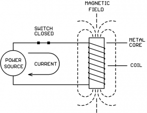
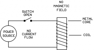
You might have built an electromagnet in high school science class and used it to pick up small metal objects. An electromagnet is a coil of wire wound around a metal core. When the coil of wire is hooked to an electrical power source and current flows through the coil, a magnetic field is produced which surrounds the coil and the core:
While the electromagnet is energized, any metal objects which come close will be physically pulled towards core.
When the switch is opened, the current flow stops and the magnetic field disappears. When the magnetic field disappears, nearby metal objects are no longer attracted to the core:
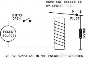
We now place a pivoted metal arm (armature) above the electromagnet, and we connect a spring to keep the armature pulled away from the electromagnet under “normal” (electromagnet de-energized) conditions:
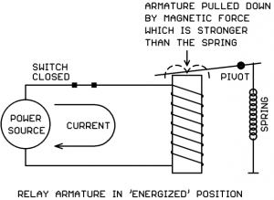
If we now energize the coil, the magnetic field will overcome the spring force and pull the armature down:
So… we have an armature which we can move up and down by de-energizing or energizing the electromagnet coil. What do we do with it?
We use the moving armature to open and close electrical contacts which are separate from the coil circuit. We can do it like this:
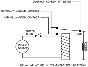
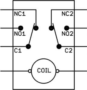
In this example, we’re using the metal armature itself as the “Common” or “Wiper” for a double-throw switch. The tip of the armature makes contact with one of two possible points depending on the position of the armature.
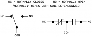
When the relay is de-energized, the armature is up and the wiper makes connection with the “Normally Closed” (NC) contact.
When the relay is energized, the armature is down and the wiper makes connection with the “Normally Open” (NO) relay contact:
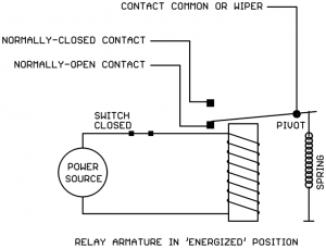
This example relay would be known as a “Single Pole, Double Throw” (SPDT) or “1 Pole, Double Throw” (1PDT) relay. It has one set of contacts (1 Pole) with both Normally Open and Normally Closed (Double Throw) connections.
Relays can have more than one set of contacts (poles). In the next example, the metal armature is not part of the electrical circuit but instead moves a plastic connector that activates two sets of contacts:
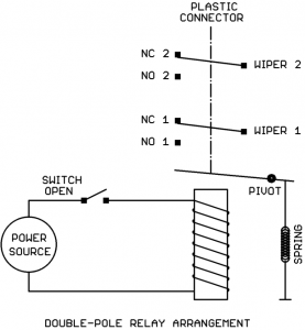
This would be known as a “Double Pole, Double Throw” (DPDT) or “2 Pole, Double Throw” (2PDT) relay.
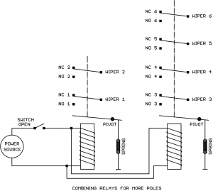
The number of poles (contact sets) can be expanded (3PDT relays, 4PDT relays etc.). Typically 4 poles is the largest relay we would see in an HVAC control panel. If you need more than 4 poles in a relay, you would probably use two relays with the coils wired together in parallel. Shown below are a DPDT relay and a 4PDT relay wired together to create 6PDT relay action:
Electrical Ratings of a Relay
The coil of a “classic” relay (no electronics) is typically rated for a specific voltage and either AC or DC operation but not both.
There are some modern relays (like Functional Devices “Relay In A Box”) that contain electronic circuits that allow the coil to operate over a range of voltages and either AC or DC operation.
If in doubt, the relay’s datasheet should clearly spell out the acceptable voltage range for the coil and whether it’s AC only, DC only, or AC/DC compatible.
Relay coils are generally tolerant of some variation in the coil voltage, a typical datasheet specification is 80% – 120% of rated coil voltage. So if a 24V transformer is “running a little hot” (putting out maybe 27V) or there is a bit of voltage drop in the coil connecting wires (maybe the coil is only getting 22V) the relay will still function just fine.
The relay contacts will have ratings for the maximum voltage allowed and the maximum current allowed. Sometimes there are multiple ratings depending on the type of load being switched (for a motor load sometimes the contacts are rated in horsepower for example). The circuit being switched by the contacts should not put more voltage or current on the contacts than allowed by the datasheet.
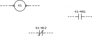
Relay Symbols Used in Wiring Diagrams
The relay coil may be drawn several different ways:
![]()
The relay contacts are typically shown one of two ways:
Relays go by several possible names on an electrical drawing:
‘R’ (not a great idea since resistors can have this designation too)
‘RL’ (better)
‘RLY’ (better still)
‘K’ (Where did this come from? We don’t know. But it’s widely used!)
If there are multiple relays, the name will be followed by a number or a letter as in RLY1, RLY2, RLY3 or RLYA, RLYB, RLYC. There might be a hyphen (-) between the name and number or letter too. There is no specific standard on how relays must be named.
Sometimes the relay is shown as a single assembly with coil and contacts arranged in a rectangle:
But sometimes the coil and the contacts are scattered around the drawing:
Relay Terminal Numbering
Unfortunately there does not seem to be a standard for the terminal numbering on relays.
Most of the relays we use in HVAC panels plug into a base socket. The pins/blades of the relay have assigned numbers and then the bases they plug into have assigned numbers on the screw terminals. If the same brand of relay and base are used together, the blade numbers usually match the terminal numbers on the base. If, however, different brands of relay and base are used together, the blade numbers may not match the base terminal numbers even though the two parts are physically compatible (example: IDEC SH3B-05 relay plugged into Omron PTF11A base). It’s a good idea to use the same brand of relay and base to avoid confusion.
Some electronic relays such as Functional Devices “Relay In A Box” have color-coded flying leads rather than screw terminals. Consult the device datasheet to determine the function of each color-coded lead.
Functions a Relay Can Perform
So what useful functions can a relay perform?
- Use a low voltage and/or low current signal (on the coil) to switch a large voltage and/or large current circuit (on the contacts).
- Use a DC signal (on the coil) to switch an AC circuit (on the contacts) or vice-versa.
- Use one signal (on the coil) to switch multiple circuits (multi-pole contacts).
- Invert the sense of a signal (using the Normally Closed contact).
- Use a signal from one circuit (on the coil) to switch another circuit (on the contacts) where the two circuits are not allowed to have any direct electrical connection.
- Use one signal (on the coil) to switch between two alternate loads (on the contacts).
- Various combinations of the above.
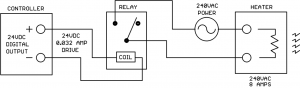
The example below demonstrates a relay performing a combination of several of the above functions. A low voltage, low current control signal from a controller is switching a high voltage, high current load on and off. The relay is also allowing a DC control signal to switch an AC load. There is also electrical isolation between the drive circuit and the load circuit so that the controller is protected from the high voltage 240V power source:
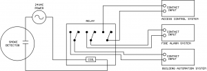
In the next scenario a smoke detector signal is being sent to three different systems simultaneously while maintaining isolation between the systems to make sure there is no unintended interaction between the systems:
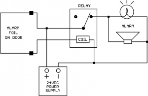
Here is an application where we want to reverse the sense of an electrical signal. We have a foil alarm loop glued to a glass door. When the foil is intact (current flowing through foil) we want to hold off the Alarm light and horn. When the foil is broken (current flow stops) we want to energize the Alarm light and horn. We can get the reverse action we want by using the Normally Closed contact on the relay:
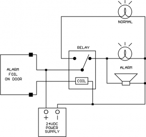
Let’s see how we can use both the N.O. and N.C. contacts to get “alternate action” between two loads. We decide that in addition to the ALARM light, we also want a NORMAL light for our alarm circuit that is on when the foil connection is intact. So we want the action of the NORMAL and ALARM lights to alternate, one or the other is on at any time, but never both at the same time. We can get this alternate action by adding the NORMAL light to the N.O. relay contact:
You may begin to see how versatile relays are. Even with all the high-tech electronics in control panels, relays will be with us for a long time to come. The operation is easy to understand and they can be used for many different applications.
Magnetic Latching Relays
There is a special class of relays known as “magnetic latching relays.” These relays contain one or more small permanent magnets which hold the armature in the last commanded position when the coil drive is removed. When a coil drive signal is applied, the magnetic field from the coil is stronger than the permanent magnets and can thus move the armature to the opposite position in spite of the permanent magnet’s presence.
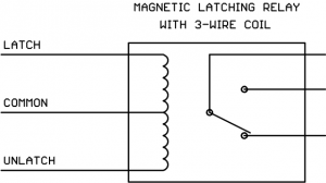
Magnetic latching relays must have two coil drive commands, Latch and Unlatch. Some relays accomplish this with two separate coil windings and two command leads:
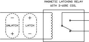
Other magnetic latching relays have just two coil wires, but the polarity of the applied DC drive determines whether the command is Latch or Unlatch:
The Latch and Unlatch drive signals are typically meant to only be momentary, you normally would not leave either signal on the coil continuously.
Magnetic latching relays are frequently used in lighting circuits. One example is the popular General Electric RR7 lighting relay.
Wrap-Up
Some points to remember about relays:
- Make sure that the relay coil voltage and AC/DC rating matches the coil drive signal in the application circuit.
- Some relays are available with a “coil energized” light built in. If any troubleshooting has to be done on the panel, these lights can be very helpful.
- Some relays are available with a manual override button built in. If any troubleshooting has to be done on the panel, these override buttons can be very helpful.
- Make sure that the relay contact voltage and current ratings are at least as high as the volts and amps that will be applied by the application circuit. If possible, use contacts rated higher than the volts and amps that will be applied.
- If you need more poles than are available on one relay, you can use multiple relays with the coils connected in parallel.
Using a Multimeter Series – Resistance Measuring Basics
“Resistance is futile, Buwhahaha” exclaimed the villain, rubbing his hands together in glee as our hero struggled to free himself from the ropes that bound him.
Yep, we’ve all seen those Grade B movies. Maybe in that situation resistance is futile, but in the world of electronics and HVAC controls resistance (electrical resistance) is very useful!
Designing selected values of resistance into the appropriate points of circuits lets us control the voltages and currents so the circuits perform as desired. The most popular forms of temperature sensors used in HVAC (RTDs and thermistors) operate by varying their electrical resistance as temperature changes. Resistors are also frequently used to convert the 4-20 mA signal from a transmitter into a 1-5V or 2-10V signal for controller inputs.
Electrical resistance is measured in units of Ohms. When resistance gets into values larger than 1000 ohms it may also be expressed in Kilohms or just ‘K’ for short (50K = 50,000 ohms). The symbol for resistance on electrical diagrams looks like this:
We’ll be measuring resistance with the Ohms function of our “multimeter” which can measure volts, current, resistance, and possibly other things too (frequency, capacitance, temperature with accessory probe, etc.). When the multimeter is set to the Ohms function, it may be referred to as an “ohmmeter.”
Plug the Meter Leads Into the Correct Meter Jacks
Shown below is a typical multimeter face layout. This is an actual meter Kele uses in our internal training classes. Note that your multimeter controls may be arranged somewhat differently or completely differently:
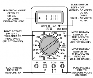
To read resistance, plug the black meter lead into the COM jack and plug the red meter lead into the V/ohm jack.
Set the Meter Selector to Ohms
The meter selector switch has different major areas for choosing whether you want to read voltage, current, resistance (ohms), or possibly other things. You need to move the selector switch to one of the positions in the Ohms area (left side of selector knob on our example meter).
Set Meter Range (Unless You Have an Auto-Ranging Meter)
Our example meter has different resistance ranges to choose from based on the maximum resistance you expect to measure. Always choose the smallest range that’s higher than the highest resistance you are expecting to measure. For example, if you are going to measure a resistance you think should be around 10K (10,000 ohms) then on the meter you would select the 20K range (because the 10K we want to check is higher than the next lower range which is 2K).
If you accidentally select a lower range than the resistance you are trying to measure, the meter won’t be damaged. You’ll get some kind of “overrange” indication on the display. This can vary from meter to meter. Sometimes it’s a row of horizontal dashes, sometimes it’s “OL” for overload, or maybe something completely different.
If your meter has an Auto-Ranging function you don’t have to worry about setting the range, the meter will figure it out for you. It will automatically step through the different ranges until it finds the lowest range that does not result in an over-range condition.
Auto-Ranging is very handy. The down side is that it can take the meter longer to display a final stable resistance reading because it has to trail-and-error each time to find the right range. A fixed-range meter manually set to the correct range will stabilize to a usable reading faster since it doesn’t have to experiment to find the correct range.
If the Resistor Is Connected In A Circuit, Disconnect At Least One End of the Resistor Before Taking A Measurement
If the resistor is connected in a circuit, at least one end of the resistor must be disconnected from the circuit before connecting the meter probes. If the resistor is left connected to other devices at both ends, you will be measuring the “equivalent resistance” of other circuit components in parallel with the resistor of interest. This will give a false reading that is lower than the actual resistor value.
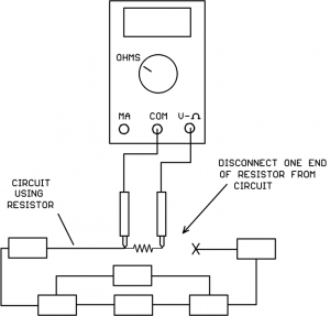
It would also be a good idea to have the circuit powered down even though one end of the resistor is disconnected. The connected end of the resistor could be attached to a live voltage or current source and bad things could happen if the probes slipped.
Place the Meter Probes Across The Resistance To Be Measured
Remember to keep your fingers on the insulated probe handles, don’t touch the metal probe tips with your fingers. Your body is a resistor from hand-to-hand too, and if you grab both metal probe tips and try to read a high resistance value, your body resistance in parallel will introduce a measurement error.
If the display shows an over-range condition, just move the meter ohms selector to the next higher range and try again.
Special Notes On Temperature Sensor Resistance Measurements
If you try to measure the resistance of a thermistor or RTD temperature sensor with a long wire run attached, you may find that the readings jump around on the display. This is caused by that long wire run acting as an antenna and picking up 60 Hz power line noise:
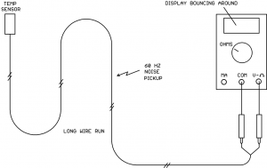
Some meters may have better noise filters than others, if you have more than one model meter available you might try them all to see which is better at noise rejection.
If the resistance value is jumping around, look for the minimum value that ever shows up on the display and the maximum value that ever shows up on the display. Chances are that the true resistance value will be approximately halfway between those two values.
You might also notice that when you put the meter probes on the thermistor or RTD sensor, the resistance value starts to slowly move (up for RTDs, down for NTC thermistors). It’s unlikely (although remotely possible) that you have an unstable sensor, it’s more likely you are seeing the effects of self-heating in the sensor.
The ohmmeter passes a small current through the sensor resistance in order to measure it. This small current causes a slight heating of the sensor material. Since temperature sensors are specifically designed to give large resistance changes with temperature change, this self-heating shows up as a slow resistance change:
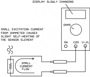
This is nothing to worry about and does not mean that the sensor is bad. The initial sensor resistance value (before self-heating takes effect) more accurately represents the temperature of the medium being measured by the sensor.
Temperature sensors with a small thermal mass and slow-moving media are more likely to exhibit self-heating effects than sensors with a large thermal mass and swiftly moving media. For example, a chip sensor sitting up in the air on two thin wires inside a wall-mount room housing will exhibit more self-heating effect than a duct sensor potted in the end of a metal tube placed in the moving air stream inside a duct.
Continuity Checks Using An Ohmmeter
Sometimes you simply want to know whether two points in a control panel or on a module terminal block are connected directly together. The ohmmeter is an excellent tool for doing continuity checks.
To perform a continuity check:
- Make sure the circuit is powered off.
- Place the ohmmeter probes on the two points to be checked.
- If the resistance is less than 1 ohm, the two points are very likely directly connected.
Why wouldn’t the resistance read zero ohms if the points were directly connected? Because all conductors icluding the ohmmeter test leads have some electrical resistance. You can prove this by shorting the ohmmeter test probes directly together and observing the display, it will show a non-zero (but very small) resistance value.
Take-Away Points
- If the resistance to be measured is mounted in a circuit, disconnect at least one end of the resistor from the circuit before measuring .
- Noise pickup on long wire runs can make the resistance value jump around on the meter. Look for the lowest and highest displayed values and take the midpoint between the two as the true value. Try a different meter to see if it has better noise filtering.
- Slowly changing temperature sensor resistance after connecting the meter is probably self-heating of the sensor element and not a bad sensor.
- When taking continuity measurements with an ohmmeter, don’t expect to read 0.00 ohms across two connected points. Any value less than 1 ohm is a good indication the points are directly connected.
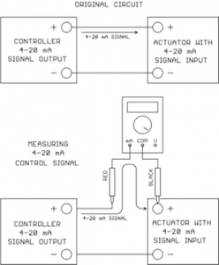
Using a Multimeter Series – Current Measuring Basics
If you are involved in installing or troubleshooting HVAC systems, sooner or later you will be taking electrical current measurements. This tutorial will discuss the basics of how to take those current measurements.
Current is measured in units of amperes, usually abbreviated to simply “amps.” When working with small currents (less than 1 amp) it may be more convenient to describe current in “milliamps,” typically abbreviated as “mA.”
When you see the term “milliamp” or “mA” this means 1/1000 of an ampere. For example:
4 mA = 4/1000 amps = 0.004 amps
20 mA = 20/1000 amps = 0.020 amps
You might be measuring AC (alternating current) or you might be measuring DC (direct current) depending on the situation. AC current is constantly reversing directions whereas DC current is always flowing in the same direction.
Very likely you will be taking current measurements for one of two reasons:
- Measuring how much current a load draws from its supply (amps or mA, AC or DC).
- Measuring a 4-20 mA control signal value (always DC).
Amp-Clamp Ammeter Versus Multimeter
If a lot of your work is done on high-current AC power circuits, an “Amp Clamp” ammeter will be very useful. An amp clamp ammeter has spring-loaded jaws that simply snap around a conductor (no electrical connection required) and the built-in display (analog or digital) reads the amps of current flowing through the conductor:
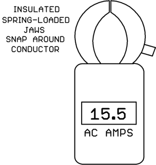
Amp-clamp ammeters are convenient, but they have some limitations:
- Typically an amp-clamp only measures AC amps; it can’t measure DC amps. (There are amp-clamps with a special kind of sensor known as a Hall Effect sensor which can measure DC amps, but these are not typical of most amp-clamps).
- The range covered is usually high (hundreds of amps) so the accuracy on small amp values is poor.
If you are measuring relatively low value AC currents or DC currents, you will likely be using the amps/mA measurement function of a multimeter. A multimeter can measure other quantities besides amps but today we are just concentrating on amp/milliamp current measurements.
Shown below is a typical multimeter face layout. This is an actual meter Kele uses in our internal training classes. It’s a few years old but the functionality of the controls is the same as a modern multimeter. Note that your multimeter controls may be arranged somewhat differently or completely differently. No one likes to do it, but you might want to actually read your multimeter instruction manual if it hasn’t been thrown away/lost by now!
To read current, plug the black meter lead into the COM jack and plug the red meter lead into the mA or 10A jack. Using the mA jack, you can measure currents up to 200 mA on this particular meter. Other model meters may have higher mA ranges available. If you want to measure currents above 200 mA on this meter, you would move the red meter lead to the 10A jack.
Be aware of meter probe properties in the mA/amp mode!
When the meter probes are plugged into COM and mA/amps jacks, the meter’s internal resistance is very low, just a fraction of an ohm. In the current mode, the probe-to-probe path through the meter looks almost like a straight piece of wire!
This has important implications. If you put the current meter probes across a power source, you will short out the power source! This makes sense if the probe-to-probe path looks like a straight piece of wire, right?
Many power sources have the capability to produce very large fault currents if their output terminals are shorted directly together. If you do this with your current meter probes, very large currents can flow through the meter!
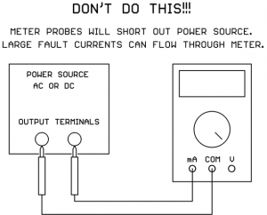
Because it’s so easy to do this accidentally, most meter manufacturers put an internal fuse in series with the meter’s mA/amp jacks. In that case, hopefully the fuse will blow and protect the meter and the power source. Still, it’s a pain to open up the meter, locate the blown fuse, and replace it.
Some very cheap meters do not have a fuse in series with the mA/amp jacks. If you send large fault currents through one of these cheap meters, the foil on the circuit board will blow apart in lieu of a fuse, rendering the meter a candidate for the trash can. Hopefully your meter does have internal fuses on the mA/amps jacks.
Set the Meter Selector to mA
The meter selector switch has different major areas for choosing whether you want to read voltage, current, resistance (ohms), or possibly other things. You need to move the selector switch to one of the positions in the mA area (lower right area on our example meter). If you are measuring large currents (amps instead of mA) the meter selector may have a separate position for that, or it may still use the mA position since there is a separate jack for amps. Check your meter’s user guide. Our example meter above still uses the selector switch set to mA even though we are using the 10A jack for large currents.
Set Meter Range (Unless You Have an Auto-Ranging Meter)
Our example meter has different current ranges to choose from when using the mA jack based on the maximum current you expect to measure. Choose the smallest range that’s above the highest current you are expecting to measure. If you are not sure what range the current will be, start on the highest range and take a measurement. Then if you can move down to a lower meter range, it will give you better accuracy.
If you accidentally select a lower range than the current you are trying to measure, the meter won’t be damaged unless you put a really large fault current through that blows the fuse. Typically you’ll get some kind of “overrange” indication on the display. This can vary from meter to meter. Sometimes it’s a row of horizontal dashes, sometimes it’s “OL” for overload, or maybe something completely different.
If your meter has an Auto-Ranging function you don’t have to worry about setting the range, the meter will figure it out for you. It usually starts on the most sensitive range and, if it sees an over-range condition, moves to the next higher range etc. until it finds the most sensitive range that does not result in an over-range condition.
Auto-Ranging is very handy. The down side is that it can take the meter longer to display a final stable current reading because it has to trial-and-error each time to find the right range. A fixed-range meter manually set to the correct range will stabilize to a usable reading faster since it doesn’t have to experiment to find the correct range.
Set Meter for AC or DC As Needed
If you set the meter to read DC mA and put the probes in a circuit with AC current, the meter will read essentially zero mA (the readout might jump around the zero reading a bit).
If you set the meter to read AC current and put the probes in a circuit with DC current, the meter display will jump up momentarily then “coast” back down to essentially zero current over time.
So be careful – an incorrect AC/DC meter setting will give completely bogus results!
If you are probing a “mystery circuit” and you’re not sure whether the current between two points is AC or DC, you can try both settings on the meter to see which gives you a non-zero value.
It’s Time To Place the Meter Probes in the Circuit
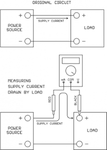
Now this is very important: to take a current measurement, you must disconnect an existing wire in the circuit and connect the meter current probes to take the place of the original connection.
The idea is that you must make the current that would normally flow directly between the two points take a detour and flow through your current meter on the way to its destination:
Remember to keep your fingers on the insulated probe handles, don’t touch the metal probe tips with your fingers just in case the connection contains high voltage. If you have jumper wires with alligator clips, these can be handy for connecting the meter probes into the circuit hands-free.
We’ve shown the current meter connected at the load in the drawings above, but it could just as easily have been connected at the power source/signal source end instead.
In the case of AC current there is no polarity to worry about, the signal will always read positive on the display no matter which way the probes are placed.
In the case of DC current, the red probe should go on the more positive point and the black probe should go on the more negative point. But if you should get it backwards no harm is done, the meter will just display a negative current value, the magnitude of the reading will still be correct and you will know that the point with the black probe is actually the more positive point.
If the display shows an over-range condition, just move the meter current selector to the next higher range and try again.
Average-Reading Versus True-RMS AC current meters
Not all current meters are created equal when it comes to measuring AC current. There are two different measurement techniques in use.
“Average-Reading” AC current meters only give a correct reading if the AC current is a sine wave. Less expensive meters tend to use the average-reading measurement technique.
“True-RMS” AC current meters will give a correct reading no matter what the wave shape (does not have to be a sine wave). This technique is typically reserved for the more expensive meters.
True-RMS current readings are based on what heating effect the current would have if passed through a resistance. The fact is that many AC-to-DC power supplies draw their AC supply current in short, high-current pulses which are not a sine wave. Since the hookup wire has resistance, and fuses are designed to open based on heating of the fuse element, True-RMS current measurements are more meaningful for applying the correct wire size and fuse size on an AC-to-DC power supply input. True-RMS current meters are therefore preferable over average-reading current meters.
Final Thoughts
The most common complaint from the field is that a current meter is reading zero. The most common problems are:
- The meter selector switch is not set for current (mA/amps).
- The meter leads are not plugged in the correct jacks (COM and mA/amps).
- The internal meter fuse is blown.
- The meter’s AC/DC switch is set opposite to the type of current actually present.